단변량 시계열 데이터 예측하기

문제를 단순하게 하기 위해서 우선 한 종류의 데이터만 사용해서 예측을 진행해 보겠습니다.

아래의 코드를 이전에 작성한 코드에 이어서 작성합니다.

온도 데이터 추출

uni_data = df['T (degC)']
uni_data.index = df['Date Time']
print(uni_data.head())

Date Time
01.01.2009 00:10:00   -8.02
01.01.2009 00:20:00   -8.41
01.01.2009 00:30:00   -8.51
01.01.2009 00:40:00   -8.31
01.01.2009 00:50:00   -8.27
Name: T (degC), dtype: float64

이제 온도 데이터만 추출되어서 날짜-시간과 온도, 두 개의 열 (column)을 갖는 데이터 (uni_data)를 얻었습니다.

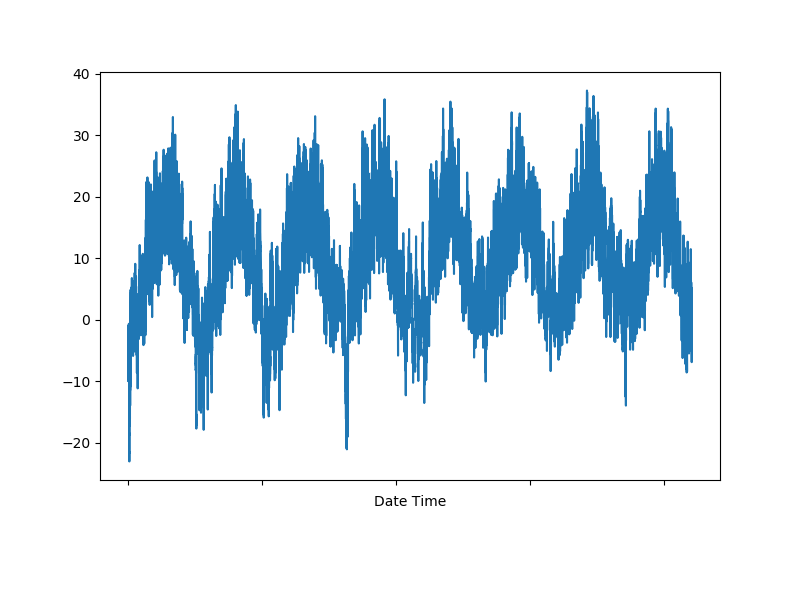
uni_data.plot(subplots=True)
plt.show()

시간에 따른 온도의 변화를 그래프로 나타내보면 아래의 그림과 같습니다.

표준화 (Standardization)

온도 데이터에 대해서, 평균을 빼고 표준편차로 나누어줌으로써 표준화를 진행합니다.

uni_data = uni_data.values
uni_train_mean = uni_data[:TRAIN_SPLIT].mean()
uni_train_std = uni_data[:TRAIN_SPLIT].std()
uni_data = (uni_data - uni_train_mean) / uni_train_std  # Standardization

print(uni_data)

[-1.99766294 -2.04281897 -2.05439744 ... -1.43494935 -1.55883897 -1.62715193]

표준화된 데이터가 출력됩니다.

첫번째 예측

이제 단변량 모델을 위한 데이터를 생성합니다.

우선 20개의 온도 관측치를 입력하면 다음 시간 스텝의 온도를 예측하도록 합니다.

univariate_past_history = 20
univariate_future_target = 0

x_train_uni, y_train_uni = univariate_data(uni_data, 0, TRAIN_SPLIT,
                                         univariate_past_history,
                                         univariate_future_target)
x_val_uni, y_val_uni = univariate_data(uni_data, TRAIN_SPLIT, None,
                                     univariate_past_history,
                                     univariate_future_target)

print('Single window of past history')
print(x_train_uni[0])
print('\n Target temperature to predict')
print(y_train_uni[0])

Single window of past history
[[-1.99766294]
[-2.04281897]
[-2.05439744]
[-2.0312405 ]
[-2.02660912]
[-2.00113649]
[-1.95134907]
[-1.95134907]
[-1.98492663]
[-2.04513467]
[-2.08334362]
[-2.09723778]
[-2.09376424]
[-2.09144854]
[-2.07176515]
[-2.07176515]
[-2.07639653]
[-2.08913285]
[-2.09260639]
[-2.10418486]]

Target temperature to predict
-2.1041848598100876

위의 출력 결과는 univariate_data() 함수가 만든 20개의 과거 온도 데이터와 1개의 목표 예측 온도를 나타냅니다.

아래의 코드를 통해 이 데이터들을 그래프로 플롯하기 위한 함수를 만듭니다.

def create_time_steps(length):
    return list(range(-length, 0))


def show_plot(plot_data, delta, title):
    labels = ['History', 'True Future', 'Model Prediction']
    marker = ['.-', 'rx', 'go']
    time_steps = create_time_steps(plot_data[0].shape[0])
    if delta:
        future = delta
    else:
        future = 0

    plt.title(title)
    for i, x in enumerate(plot_data):
        if i:
            plt.plot(future, plot_data[i], marker[i], markersize=10, label=labels[i])
        else:
            plt.plot(time_steps, plot_data[i].flatten(), marker[i], label=labels[i])
    plt.legend()
    plt.axis('auto')
    plt.xlim([time_steps[0], (future+5)*2])
    plt.xlabel('Time-Step')
    return plt

create_time_steps() 함수는 데이터의 길이를 이용해서 시간 스텝 값들을 만듭니다.

(참고: Python 내장함수 - list)

그리고 show_plot() 함수는 이 온도 데이터들을 matplotlib 그래프로 반환합니다.

(참고: Matplotlib - 파이썬 그래프 플롯 라이브러리)

그리고 앞에서 만든 훈련용 데이터 [x_train_uni[0], y_train_uni[0]]를 그래프로 나타냅니다.

show_plot([x_train_uni[0], y_train_uni[0]], 0, 'Sample Example').show()

결과는 아래와 같습니다.

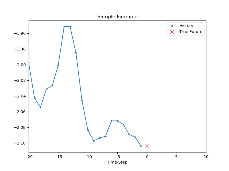
파란 마커가 20개의 과거 온도 데이터, 빨간 마커가 예측해야 할 미래의 (실제) 온도 데이터를 나타냅니다.

이제 첫번째 예측을 해보겠습니다.

def baseline(history):
    return np.mean(history)


show_plot([x_train_uni[0], y_train_uni[0], baseline(x_train_uni[0])], 0, 'Sample Example').show()

baseline 함수는 과거 20개의 데이터를 받아서 그 평균을 반환하는 함수입니다.

이 평균값을 첫번째 예측으로 사용해서 그래프로 나타내보겠습니다.

(참고: NumPy 다양한 함수들 - numpy.mean)

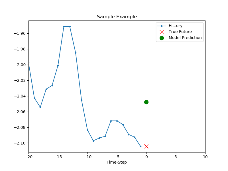
녹색 마커는 과거 온도 데이터의 평균값을 이용해서 예측한 지점을 나타냅니다.

실제 데이터와 꽤 차이가 있음을 알 수 있습니다.

다음 페이지에서는 순환 신경망 (recurrent neural network)을 이용해서 미래의 데이터를 예측해 보겠습니다.

지금까지 작성한 코드는 아래와 같습니다.

import tensorflow as tf
import matplotlib as mpl
import matplotlib.pyplot as plt
import numpy as np
import os
import pandas as pd

mpl.rcParams['figure.figsize'] = (8, 6)
mpl.rcParams['axes.grid'] = False

zip_path = tf.keras.utils.get_file(
    origin='https://storage.googleapis.com/tensorflow/tf-keras-datasets/jena_climate_2009_2016.csv.zip',
    fname='jena_climate_2009_2016.csv.zip',
    extract=True)
csv_path, _ = os.path.splitext(zip_path)

df = pd.read_csv(csv_path)
# print(df.head())
# print(df.columns)


def univariate_data(dataset, start_index, end_index, history_size, target_size):
    data = []
    labels = []

    start_index = start_index + history_size
    if end_index is None:
        end_index = len(dataset) - target_size

    for i in range(start_index, end_index):
        indices = range(i - history_size, i)
        # Reshape data from (history_size,) to (history_size, 1)
        data.append(np.reshape(dataset[indices], (history_size, 1)))
        labels.append(dataset[i+target_size])
    return np.array(data), np.array(labels)


TRAIN_SPLIT = 300000
tf.random.set_seed(13)

uni_data = df['T (degC)']
uni_data.index = df['Date Time']
# print(uni_data.head())

# uni_data.plot(subplots=True)
# plt.show()

uni_data = uni_data.values
uni_train_mean = uni_data[:TRAIN_SPLIT].mean()
uni_train_std = uni_data[:TRAIN_SPLIT].std()
uni_data = (uni_data - uni_train_mean) / uni_train_std  # Standardization

# print(uni_data)

univariate_past_history = 20
univariate_future_target = 0

x_train_uni, y_train_uni = univariate_data(uni_data, 0, TRAIN_SPLIT,
                                           univariate_past_history,
                                           univariate_future_target)
x_val_uni, y_val_uni = univariate_data(uni_data, TRAIN_SPLIT, None,
                                       univariate_past_history,
                                       univariate_future_target)

# print('Single window of past history')
# print(x_train_uni[0])
# print('\n Target temperature to predict')
# print(y_train_uni[0])


def create_time_steps(length):
    return list(range(-length, 0))


def show_plot(plot_data, delta, title):
    labels = ['History', 'True Future', 'Model Prediction']
    marker = ['.-', 'rx', 'go']
    time_steps = create_time_steps(plot_data[0].shape[0])
    if delta:
        future = delta
    else:
        future = 0

    plt.title(title)
    for i, x in enumerate(plot_data):
        if i:
            plt.plot(future, plot_data[i], marker[i], markersize=10, label=labels[i])
        else:
            plt.plot(time_steps, plot_data[i].flatten(), marker[i], label=labels[i])
    plt.legend()
    plt.axis('auto')
    plt.xlim([time_steps[0], (future+5)*2])
    plt.xlabel('Time-Step')
    return plt


# show_plot([x_train_uni[0], y_train_uni[0]], 0, 'Sample Example').show()


def baseline(history):
    return np.mean(history)


show_plot([x_train_uni[0], y_train_uni[0], baseline(x_train_uni[0])], 0, 'Sample Example').show()

이전글/다음글

이전글 : 날씨 데이터셋

다음글 : 순환 신경망 사용하기

공유하기