5. AND 로직 연산 학습하기

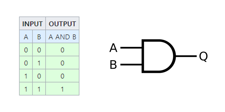
AND 연산은 논리 연산 (Logic operation)의 한 종류로 위의 그림과 같이 두 상태가 모두 참 (True, 1)일 때 참이고,

둘 중 하나라도 거짓 (False, 0)이라면 거짓이 되는 연산입니다.

전기 신호가 0과 1로 구성되어 있는 디지털 회로에서는 트랜지스터 게이트의 조합으로 구현할 수 있습니다.

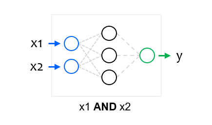
위 그림은 두 개의 입력값을 받고, 하나의 값을 출력하는 간단한 인공신경망 (Artificial Neural Network)을 나타냅니다.

이제 TensorFlow를 이용해서 두 입력값에 대해 AND 논리 연산의 결과를 출력하는 신경망을 구현해보겠습니다.

1) 훈련 데이터 준비하기

import tensorflow as tf
from tensorflow import keras
import numpy as np

tf.random.set_seed(0)

# 1. 훈련 데이터 준비하기
x_train = [[0, 0], [0, 1], [1, 0], [1, 1]]
y_train = [[0], [0], [0], [1]]

우선 tf.random 모듈의 set_seed() 함수를 사용해서 랜덤 시드를 설정했습니다.

예제에서 x_train, y_train은 각각 훈련에 사용할 입력값, 출력값입니다.

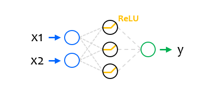
2) Neural Network 구성하기

# 2. 모델 구성하기
model = keras.Sequential([
    keras.layers.Dense(units=3, input_shape=[2], activation='relu'),
    keras.layers.Dense(units=1)
    ])

tf.keras 모듈의 Sequantial 클래스는 Neural Network의 각 층을 순서대로 쌓을 수 있도록 합니다.

tf.keras.layers 모듈의 Dense 클래스는 완전히 연결된 뉴런층을 구성합니다.

두 개의 Dense를 사용해서 아래 그림과 같은 구조의 신경망을 구성했습니다.

은닉층 (Hidden layer)의 활성화함수로 ReLU (Rectified Linear Unit)를 사용했습니다.

3) Neural Network 컴파일하기

# 3. 모델 컴파일하기
model.compile(loss='mse', optimizer='Adam')

손실 함수로 ‘mse’를, 옵티마이저로 ‘Adam’을 지정했습니다.

4) Neural Network 훈련하기

# 4. 모델 훈련하기
pred_before_training = model.predict(x_train)
print('Before Training: \n', pred_before_training)

history = model.fit(x_train, y_train, epochs=1000, verbose=0)

pred_after_training = model.predict(x_train)
print('After Training: \n', pred_after_training)

Before Training:
[[0.        ]
[0.6210649 ]
[0.06930891]
[0.6721569 ]]
After Training:
[[-0.00612799]
[ 0.00896954]
[ 0.00497065]
[ 0.9905546 ]]

tf.keras 모듈의 Model 클래스는 predict() 메서드를 포함합니다.

predict() 메서드를 이용해서 Neural Network의 예측값 (predicted value)을 얻을 수 있습니다.

Model 클래스의 fit() 메서드는 모델을 훈련하고, 훈련 진행 상황과 현재의 손실값을 반환합니다.

모델 훈련의 전후로 입력 데이터에 대한 Neural Network의 예측값을 출력하도록 했습니다.

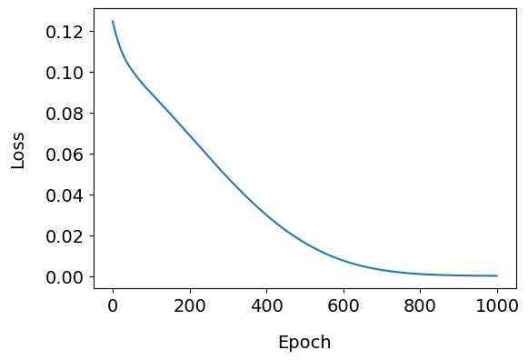
5) 손실값 확인하기

# 5. 손실값 확인하기
import matplotlib.pyplot as plt

loss = history.history['loss']
plt.plot(loss)
plt.xlabel('Epoch', labelpad=15)
plt.ylabel('Loss', labelpad=15)

plt.show()

fit() 메서드가 반환하는 손실값을 Matplotlib 라이브러리를 사용해서 시각화했습니다.

결과는 아래와 같습니다.

6) 훈련 결과 확인하기

import matplotlib.pyplot as plt
import numpy as np

plt.style.use('default')
plt.rcParams['figure.figsize'] = (6, 4)
plt.rcParams['font.size'] = 14

plt.plot(pred_before_training, 's-', markersize=10, label='pred_before_training')
plt.plot(pred_after_training, 'd-', markersize=10, label='pred_after_training')
plt.plot(y_train, 'o-', markersize=10, label='y_train')

plt.xticks(np.arange(4), labels=['[0, 0]', '[0, 1]', '[1, 0]', '[1, 1]'])
plt.xlabel('Input (x_train)', labelpad=15)
plt.ylabel('Output (y_train)', labelpad=15)

plt.legend()
plt.show()

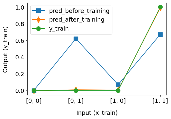
Matplotlib 라이브러리를 사용해서 훈련 전후의 입력값, 출력값을 나타냈습니다.

간단한 신경망에 대해 1000회의 훈련이 이루어지면, 네가지 경우의 0과 1 입력에 대해 1% 미만의 오차로

AND 연산을 수행할 수 있음을 확인할 수 있습니다.

전체 예제 코드

전체 코드는 아래와 같습니다.

신경망을 구성하는 과정에서 뉴런의 개수, 활성화함수, 그리고 옵티마이저를 바꿔가면서

훈련의 횟수와 정확도에 미치는 영향을 확인해 볼 수 있습니다.

import tensorflow as tf
from tensorflow import keras
import numpy as np

tf.random.set_seed(0)


# 1. 훈련 데이터 준비하기
x_train = [[0, 0], [0, 1], [1, 0], [1, 1]]
y_train = [[0], [0], [0], [1]]


# 2. 모델 구성하기
model = keras.Sequential([
    keras.layers.Dense(units=3, input_shape=[2], activation='relu'),
    # keras.layers.Dense(units=3, input_shape=[2], activation='sigmoid'),
    keras.layers.Dense(units=1)
    ])


# 3. 모델 컴파일하기
# model.compile(loss='mse', optimizer='SGD')
model.compile(loss='mse', optimizer='Adam')


# 4. 모델 훈련하기
pred_before_training = model.predict(x_train)
print('Before Training: \n', pred_before_training)

history = model.fit(x_train, y_train, epochs=1000, verbose=0)

pred_after_training = model.predict(x_train)
print('After Training: \n', pred_after_training)


# 5. 손실값 확인하기
import matplotlib.pyplot as plt

loss = history.history['loss']
plt.plot(loss)
plt.xlabel('Epoch', labelpad=15)
plt.ylabel('Loss', labelpad=15)

plt.show()

이전글/다음글

이전글 : 4. 옵티마이저 사용하기

다음글 : 6. 뉴런층의 속성 확인하기

공유하기